mist: Multispectral Image
Similarity Transformation
Version: 1.0
Release: April, 1997
Item: Documentation
RESTRICTED RIGHTS LEGEND
Use, duplication, or disclosure by the Government is subject to restrictions
as set forth in subparagraph (c)(1)(ii) of the Rights in Technical Data and
Computer Software clause at DFARS 252.227-7013 or FAR 52.227-14, as applicable.
This document describes work intended to aid in the problem of automatically
registering two images of dissimilar type. This work was performed under NASA
contract number NAS5-32357. It was performed by Sridhar Srinivasan, Carl Stevens,
Les Elkins, Radha Poovendran, and Srinivasan Raghavan.
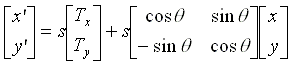
The algorithms implemented in this software attempt to determine a transformation from one image to another. The registration software can be used to register similar or dissimilar multi-sensor imagery as long as the transformation between this imagery is restricted to rotation, translation, and scaling (collectively known as a "similarity transformation"). This composite transformation can be expressed as:
where:
(x',y') is the transformed point in the second
image, image2, corresponding to (x,y) in the first image, image1,
s is the common scale by which image1 was expanded to create image2,
Tx, Ty are the units that image1 was translated
in the x and y axes,
![]() is the angle by which image1
was rotated, and
is the angle by which image1
was rotated, and
(x,y) is the source point in the original image.
The algorithms which determine the scale, translation, and rotation of the two
images are based on lines extracted from the original images. By working with
these lines rather than the images themselves, the algorithm can deal with differing
types of imagery (visible, IR, AVHRR, etc.).
The algorithm performs five steps:
Each of these will be dealt with in greater detail below.
The quality of edges obtained using any given edge detection technique is very critical to the output of the line extraction algorithm. The desirable features in an edge detection algorithm therefore include:
Canny showed that the solution to these three constraints leads to a linear match filter. From numerical optimizations, Canny also noted that an efficient approximation to the edge function is the derivative of the Gaussian,
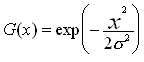
where x is the location of the edge and is the standard
deviation of the Gaussian function.
To produce the list of valid edges, the code does the following:
Once the edges are extracted, they must be converted into lines.
This is done by grouping valid edge points that lie along lines and creating
line segments. Valid lines are determined by edge density and line length.
This method generates many valid line segments, but will also generate a number
of spurious ones. Inclusion of these segments in the parameter estimation algorithms
will skew the estimated transformation parameter values. It is therefore necessary
to use thresholding operations which will eliminate as many spurious line segments
as possible. The current version of the code picks rather permissive parameters,
which nonetheless keeps the algorithm from generating many of the very small
lines.
The algorithms used in the following sections contain code that will increase
in computational cost greatly as the number of lines used increases. Thus once
the lines are generated, it is still desirable to further reduce their number.
This is done by choosing a minimum length threshold based on an examination
of the histogram. The threshold chosen by the code as it stands now is the value
one quartile from the lowest value, thus three quarters of the lines remain
after this additional restriction.
Given a set of lines from each image of the pair, we wish to
determine the rotation angle needed to rotate the lines in one image to those
in the second. This requirement is complicated by the fact that there may not
be a high degree of correspondence between the two sets of lines, and by the
possibility that the two sets of lines are at different scales and may be shifted
spatially. It is therefore desirable to use techniques based on histogram solutions,
which will give us the maximum likelihood solution for the parameter estimation
problems at hand.
The first step in computing the rotation is to determine the direction of each
line. The direction is given as the angle with respect to the x
axis, and is constrained to be between ![]() and
and  . Then, for each
line in the first image, the difference in angle to each line in the second
image is computed. This then gives us a list of the difference in direction
between all lines in the first file to all lines in the second file. While in
practice the images we have used have contained a manageable number of lines,
note that the number of values stored (number of lines above threshold length
in image one times number of lines above threshold in image two) can get very
large, and it may be desirable to increase the length threshold for some images.
. Then, for each
line in the first image, the difference in angle to each line in the second
image is computed. This then gives us a list of the difference in direction
between all lines in the first file to all lines in the second file. While in
practice the images we have used have contained a manageable number of lines,
note that the number of values stored (number of lines above threshold length
in image one times number of lines above threshold in image two) can get very
large, and it may be desirable to increase the length threshold for some images.
To analyze this list, we perform a histogram analysis of the difference values.
Since in the problem domain we are examining implies that we have at least coarse
correspondence between the image pair, we typically assume that the rotational
angle between the two images is between -10 degrees and +10 degrees. This default
can be overridden to look for rotational correlation over larger angles. We
can then build our histogram accordingly, ignoring angle differences outside
these bounds.
The optimum number of bins in the histogram is a function of the desired accuracy
(which implies a small bin size, and thus a large number of bins) and the amount
of data to be examined (with sparse data, bin sizes too small might not be filled
adequately, and thus might give spurious results, implying the need for a small
number of bins). In this implementation, 100 bins are used, giving a bin size
of
![]()
degrees per bin.
The histogram is then filtered by two passes with a (1,2,1) mean filter, and the angle value corresponding to the bin with the maximum number of entries is chosen as the rotational value. The set of lines corresponding to the second image is then rotated by the negative of this determined value for further processing. This rotation is performed about the center of the image.
Even though lines are robust enough to use as features, some
line segments in each image may be broken or missing altogether due to various
reasons (noise, poor contrast, etc.). Hence simple examination of the ratio
of scales of corresponding lines (as we examined the angles of corresponding
lines above) is insufficient to give good results. The method implemented in
this project composes the given lines into triangles, and determines the ratio
of the area of the triangles in the first image to the triangles in the second
image.
To form the triangles, the list of lines is exhaustively searched. To find a
potential triangle from the first image, three lines from that image, l1,
l2, and l3, are chosen such that their directions differ from
each other by more than some angle tolerance . In the current implementation,
is 25 degrees. This prevents excessively slivered triangles from being considered,
as they would have a small area which might skew the results. Note that we are
not looking for actual triangles in the line segments, but rather lines which
can be extended to form triangles for consideration. To find a corresponding
triangle in the second image, we find lines l1', l2', and l3'
such that l1', l2', and l3' have directions greater than
degrees apart, and which additionally fulfill the requirement that each corresponding
line in the two triangles is within some tolerance : that is, the direction
of l1 and l1' differ by less than degrees, l2 and l2'
differ by less than degrees, and l3 and l3' differ by less than
degrees. defaults to ten degrees in the current implementation. Note that for
any triangle in the first image there may be several in the second image that
fulfill these requirements.
Once two sets of lines are found, the area of the triangles they represent must
be determined. This is computed by a determinant:
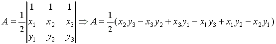
where (x1, y1), (x2, y2), and (x3,
y3) are the coordinates of the vertices of the triangle. This computation
is performed for both triangles. Since the x and y
axes in the second image are scaled by s, a triangle from the
first image with area A should have a corresponding triangle in the second
image with an area roughly equal to s2A. Thus
the square root of the ratio of a triangle's area in the second image to the
area of a corresponding triangle in the first image will be the scale factor
between these triangles. Note that since this computation depends on the triangle's
area only, it is invariant with respect to both translation and rotation. Also,
since particularly small areas in the denominator can skew the results, we ignore
small triangles.
With this computation performed on the large number of corresponding triangles
present in an image, then a large number of ratios will be available in a list.
We then perform histogram analysis as we did in the case of rotation to determine
the most common scaling factor, except the histograms are built in log space.
This factor is then used to invert the scaling in the line list from the second
image, in order to obtain a true translation estimation, as described next.
To find the translation parameters, the algorithm again builds a list of triangles as in the scaling code, this time using the derotated and descaled lines. The centroid of each triangle is generated by:
![]()
A list is then generated of all possible translations between the centers of
corresponding triangles. Again using histogram methods, we determine the x
and y values that occur the maximum number of times in
the range of interest. These are the translation values, Tx
and Ty.
With all four parameters now known, the code performs the transformation on
the second image to rotate, scale, and translate it to correspond to the first.
This section describes the function names in the C code and the parameters they take and return. In most cases, the algorithms have been discussed in the previous section.
register_images makes the calls to the supporting routines
to perform the line identification and correlation.
void register_images ( char
*in1, /* primary input file name (pgm file) */
char *in2, /* secondary input file name (pgm file)
*/
char *out, /* output file name (pgm file) */
float sigma, /* sigma for canny edge detection
*/
float min_segment, /* minimum length of poly-line
segment */
float max_distance, /* max. distance of poly line
from edge */
float thresh, /* min. line length considered */
float rotation_range, /* range of (+/-) permissible
rotation */
float scale_range, /* range of scales in percent
(+/-) 100 */
float shift_range /* range of shifts in pixels
*/
)
These parameters are primarily passed to the supporting functions. If a zero
is passed for any of the numeric parameters, then default values will be chosen.
This function also computes the desired minimum line length if it is passed
a zero for thresh (it chooses the value one quartile into the sorted list of
lengths).
compare defines a comparison function for two pointers
to floating point values. This function is used from C's built in qsort function.
int compare (const void *a, const void *b)
This function is not intended to be directly called by the user.
compute_rotation determines the rotation offset between
two sets of lines.
float compute_rotation(float *ang1, /* Array of
angles for lines in first image */
float *ang2, /* " " " " " " second " */
int dlength1, /* Number of lines from first image.
*/
int dlength2, /* " " " " second " */
float *length1, /* Length of lines from first image.
*/
float *length2, /* " " " " second " */
float thresh, /* Minimum line length considered.
*/
float range) /* Max number of degrees rot. considered
*/
The number returned is the rotation angle (in degrees).
derotate performs the derotation.
void derotate (rectlist *indata, /* Input line
endpoint list. */
rectlist *outdata, /* Destination (rotated) line
endpoint list. */
int dlength, /* Number of lines in the list. */
float rotation) /* Degrees to rotate the line list.
*/
Note that the rotation is performed with respect to the center of the image
(so the endpoints are translated by (-1/2 xsize, -1/2 ysize) before rotation,
then translated back by the same amount before storage).
differs compares two floating point numbers (angles in
degrees).
int differs (float deg1, float deg2)
The function returns one (true) if they are greater than some number of degrees
from each other, and zero (false) if they are not. The difference threshold
is defined in the routine as a constant, and is 25 in the current implementation.
This function also deals with wraparound. If it compares, for example, line
segments with angles 2 degrees and 178 degrees, it will treat them as differing
by 4 degrees rather than 176.
is_close compares two floating point numbers (angles
in degrees).
int is_close (float deg1, float deg2)
The function returns one (true) if they are within some number of degrees of
each other, and zero (false) if they are not. The difference threshold is defined
in the routine as a constant, and is 10 in the current implementation. This
function also deals with wraparound, so if it compares, for example, line segments
with angles 2 degrees and 178 degrees, it will treat them as differing by 4
degrees rather than 176.
compute_param takes a list of line endpoints and computes
the angle and length of each segment.
void compute_param (rectlist *data, /* Input line
endpoint list. */
int dlength, /* Number of line segments. */
float *length, /* Returned segment lengths. */
float *ang, /* Returned segment angle (direction).
*/
float *cosx, /* Returned cosine value of angle.
*/
float *sinx, /* Returned sine value of angle. */
float *px) /* px contains x sin ang - y cos of
ang */
This routine computes a number of numeric values for later use, as indicated
above.
rescale will rescale the line endpoints given the data
given a scaling factor.
void rescale (rectlist *indata, /* Input line endpoint
list. */
rectlist *outdata, /* Output line endpoint list.
*/
int dlength, /* Number of line segments. */
float scale) /* Scale multiplier. */
The endpoint values are scaled about the origin.
intersection will compute the intersection between the
two lines specified.
float *intersection (float sin1, /* sine of angle
of first line */
float cos1, /* cosine of angle of first line */
float p1, /* intercept representation of first
line */
float sin2, /* sine of angle of second line */
float cos2, /* cosine of angle of second line */
float p2) /* intercept representation of second
line */
While the use of sine and cosine for each angle overspecifies the line, these
numbers have already been calculated and stored, so it is more efficient to
use both. It returns the x and y values of the intersection.
max_smooth takes a histogram of values, and returns the
maximum histogram bin with the maximum value after smoothing.
int max_smooth (int *hist, /* The histogram array.
*/
int n) /* The number of histogram elements. */
The code implements a 1-2-1 filter twice (that is, ![]() )
before choosing the maximum value.
)
before choosing the maximum value.
compute_scale computes the scale between two sets of
lines.
float compute_scale(rectlist *data1, /* First line
endpoint list. */
rectlist *data2, /* Second line endpoint list.
*/
int dlength1, /* Number of segments in first line.
*/
int dlength2, /* Number of segments in second line.
*/
float *length1, /* First segment lengths. */
float *length2, /* Second segment lengths. */
float *cos1, /* First lines' cosine value of angle.
*/
float *cos2, /* Second lines' cosine value of angle.
*/
float *sin1, /* First lines' sine value of angle.
*/
float *sin2, /* Second lines' sine value of angle.
*/
float *p1, /* Contains x sin of ang - y cos of
ang */
float *p2, /* Contains x sin of ang - y cos of
ang */
float *dir1, /* Second line's direction. */
float *dir2, /* Second line's direction. */
float thresh, /* Minimum line length considered.
*/
float range) /* Scale difference considered. */
The number returned is the scale factor in percent (100.0 is no scaling).
compute_shift computes the x and y translation between
sets of lines.
float compute_shift(float *retval, /* Return val:
[0] is x, [1] is y. */
rectlist *data1, /* First line endpoint list. */
rectlist *data2, /* Second line endpoint list.
*/
int dlength1, /* Number of segments in first line.
*/
int dlength2, /* Number of segments in second line.
*/
float *length1, /* First segment lengths. */
float *length2, /* Second segment lengths. */
float *cos1, /* First lines' cosine value of angle.
*/
float *cos2, /* Second lines' cosine value of angle.
*/
float *sin1, /* First lines' sine value of angle.
*/
float *sin2, /* Second lines' sine value of angle.
*/
float *p1, /* Contains x sin of ang - y cos of
ang */
float *p2, /* Contains x sin of ang - y cos of
ang */
float *dir1, /* Second line's direction. */
float *dir2, /* Second line's direction. */
float thresh, /* Minimum line length considered.
*/
float shift_range) /* Translational difference
considered. */
The translation values are returned in retval.
image__clear clears the elements of the image data structure
for later use.
void image__clear (image *in) /* in is a pointer
to an image data type. */
image__free_char frees the space allocated to an image
with the image__allocate_char routine.
void image__free_char (image *in, /* Image pointer.
*/
unsigned char **ucmatrix) /* data pointer. */
image__allocate_char allocates a 2d matrix of characters.
unsigned char **image__allocate_char (int cc, /*
Number of columns... */
int rr) /* Number of rows. */
The function returns a pointer to the area allocated.
image__allocate_float allocates a 2d array of floating
point storage.
float **image__allocate_float (int cc, /* Number
of columns... */
int rr) /* Number of rows.... */
The routine returns a pointer to the allocates space.
image__write_pnm writes a pnm format graphics file.
int image__write_pnm (image *in, /* Image file
to write. */
char *str) /* Filename. */
The routine returns zero (false) if it cannot write the file, true otherwise.
image__read_pgm_header examines the header of a pgm (portable
greymap) format graphics file.
int image__read_pgm_header(FILE *fp, /* File pointer
to the (open) file. */
int *cc, /* Pointer to returned num of columns.
*/
int *rr, /* Pointer to returned num of rows. */
int *ncol) /* Pointer to returned num of colors.
*/
The routine returns zero (false) if it cannot read the file header, true otherwise.
It also indicates the number of columns, rows, and colors in the image through
the pointers passed to it.
image__read_pgm_image reads the data in a pgm image.
int image__read_pgm_image(image *in, /* Pointer
to the image data structure. */
char *str) /* Pointer to the filename. */
The routine returns zero (false) if it cannot read the file, true otherwise.
The actual data is returned in the image data structure.
image__alloc allocates the memory needed to read the
image data in.
int image__alloc (image *in, /* Pointer to the
image data structure. */
int nc, /* Numnber of colors in the image. */
int cc, /* Number of columns in the image.*/
int rr) /* Number of rows in the image.*/
This routine modifies the image data structures.
image__read is a wrapper to perform the read. It prints
out an informational message in the process.
int image__read(image *in, /* Pointer to the image
data structure. */
char *str) /* Pointer to the filename. */
image__free frees the allocated memory associated with
the image in question.
void image__free (image *in, /* Pointer to the
image data structure. */
image__follow follows a connected edge.
int image__follow(int i, /* location */
int j, /* location */
int low, /* Low threshold */
int cols, /* Cols in image */
int rows, /* Rows in image */
unsigned char **data, /* Keeps track of visited
points. */
unsigned char **mag) /* Gradient data (I think).
*/
This is a recursive routine, called by image__canny. It attempts to look around
in an area and track adjacent points.
image__canny performs Canny edge detection. This code
is modified from the shareware developed by the Robot Vision Group, University
of Edinburgh, U.K. by Bob Fisher, Dave Croft and A Fitzgibbon. The modifications
were made to allow it to work in our environment.
void image__canny (image *in, /* Original image.
*/
float s) /* Threshold sigma parameter. */
The results are stored in the image.
image__thin is a thinning algorithm for binary images.
See `Image Processing' by Anil K Jain (p383) for details.
void image__thin (image *in) /* in is the (binary)
image in question. */
image__split is a split function for fitting poly-lines
to a list
int image__split (LIST *in,
int n,
LIST *out,
float *d_array,
float max_dist)
The routine is called from image_trace, and is recursive.
image__trace is used to find lines.
>int image__trace(image *img,
LIST *list,
int *listlength,
int x0,
int y0,
float max_dist)
It is used by image__r2v to convert to find the lines in an image.
image__r2v performs the raster to vector conversion.
int image__r2v(image *in, /* image w/pixel val
of 0/1 for edge presence) */
float in_seg, /* Minimum segment threshold. */
float in_dist, /* Maximum distance for thresholded
points. */
rectlist *rlptr, /* The line segment endpoints.
*/
int maxl) /* Maximum number of lines. */
The routine returns the number of lines identified in the image. The line data
is returned in rlptr.
The following table documents the algorithm's results on several image pairs.
|
Original Image |
Second Image |
Perceived Rotation |
Perceived Scaling |
Perceived Translation |
|
ortho1.pgm |
ortho1_r7.pgm |
anti,7.40 |
99.50% |
3.2,2.4 |
|
ortho1_r7.pgm |
ortho1.pgm |
7.20 |
100.50% |
0.0,-0.8 |
|
ortho1.pgm |
ortho1_s95.pgm |
0.20 |
94.06% |
0.8,4.0 |
|
ortho1_s95.pgm |
ortho1.pgm |
anti,0.40 |
106.31% |
0.0,-4.0 |
|
ortho1.pgm |
ortho1_t26.pgm |
anti,0.20 |
100.10% |
26.4,-25.6 |
|
ortho1_t26.pgm |
ortho1.pgm |
anti,0.20 |
100.10% |
-25.6,22.4 |
|
ortho1.pgm |
ortho1_r7_s95.pgm |
anti, 7.00 |
99.50% |
-20.8,-0.8 |
|
ortho1_r7_s95.pgm |
ortho1.pgm |
7.00 |
100.50% |
16.8,8.0 |
|
ortho1.pgm |
ortho1_r7_t10.pgm |
anti, 7.4 |
99.30 |
-4.8,12.8 |
|
ortho1_r7_t10.pgm |
ortho1.pgm |
7.20 |
102.95% |
2.4,-12.8 |
|
ortho1.pgm |
ortho1_s95_t10.pgm |
0.20 |
94.44% |
-11.2,12.8 |
|
ortho1_s95_t10.pgm |
ortho1.pgm |
anti,0.40 |
105.88% |
11.2,-12.8 |
|
ortho1.pgm |
ortho1_r7_s95_t20.pgm |
anti,7.0 |
96.16% |
-22.4,23.2 |
|
ortho1_r7_s95_t20.pgm |
ortho1.pgm |
6.8 |
102.54% |
28.8,-16 |
Figure 1 Table of Results
Note that 'anti' rotation is counterclockwise.
Image sources: The original image is ortho1.pgm, a 1024x1024 image taken
from a grayscale orthophoto obtained from the USGS. The image of an area in
Carderock, Maryland, and is 2 meters per pixel. All other comparison images
were generated by the noted transformations:
Note that most of the results are reasonable. One of the exceptions is the case
where the comparison image was ortho1_r7_s95.pgm. In this case, the rotation
was found accurately, but the scaling was not. Curiously, when this image was
then translated as in ortho1_r7_s95_t20.pgm, the perceived scaling values were
much better. Examination of the histograms of relative ratio of areas between
the triangles used for scale determination indicates that in this set of images,
the 'correct' scale is not greatly higher than the nearby scales. Additionally,
in the images ortho1_r7_s95_t20.pgm and ortho1_r7_s95.pgm the boundaries created
by the transformation were filled in by hand separately in each case. Several
lines were found in the hand-drawn areas in the non-translated image that were
not present in the translated image, and these contributed to the ratio of areas
enough to skew the results to a different histogram bin.
In this section, the intermediate results from a single pair
of images are presented. Note that the converter we used did some odd
things in the conversion to GIF, hence the green tinge of the photos- which
were originally greyscale.
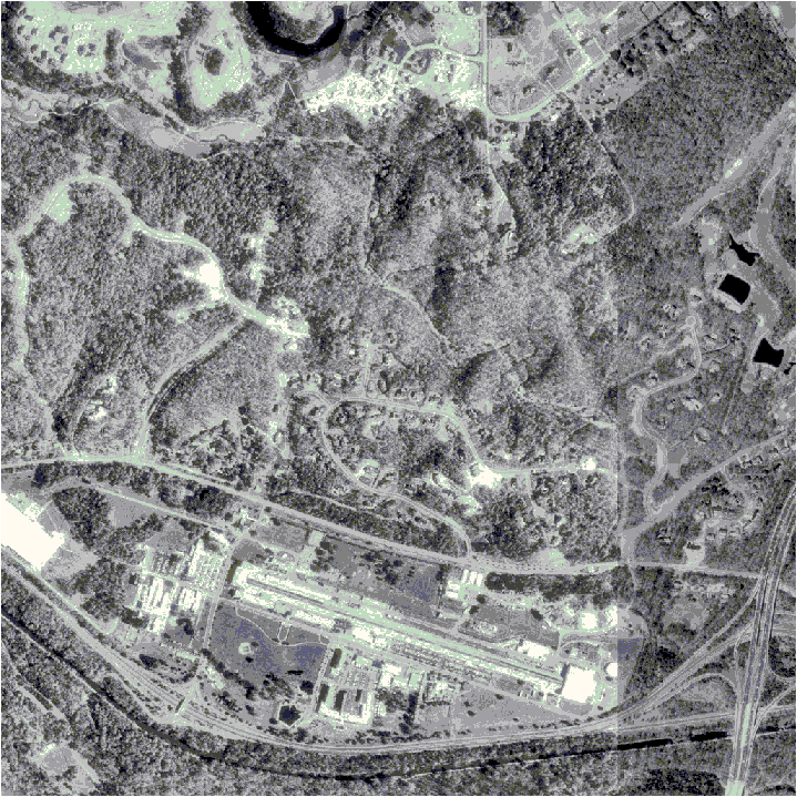
Figure 2 First source
image: ortho1.pgm
The first image, ortho1.pgm, is taken from a larger USGS orthophoto.

Figure 3 Edges in
first image
The above figure shows the edges detected by the Canny operation on the first
source image.
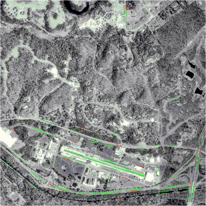
Figure 4 Lines detected
in ortho1.pgm
The lines detected in the first source image are shown above, overlaid on the
original. The lines that are below threshold are colored red, and the lines
used are in green
.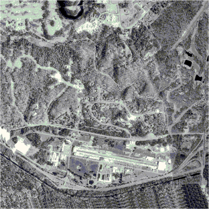
Figure 5 Second source image: ortho1_r7_s95_t20.pgm
The above image is the second source used for this test. It is a rotated, translated,
and scaled version of the original, with cloned trees filling in the areas around
the edges created by shrinking and scaling the original.
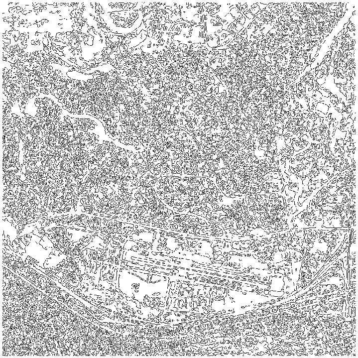
Figure 6 Edges detected
in second image
The above figure shows the edges detected by the Canny operation on the first
source image.
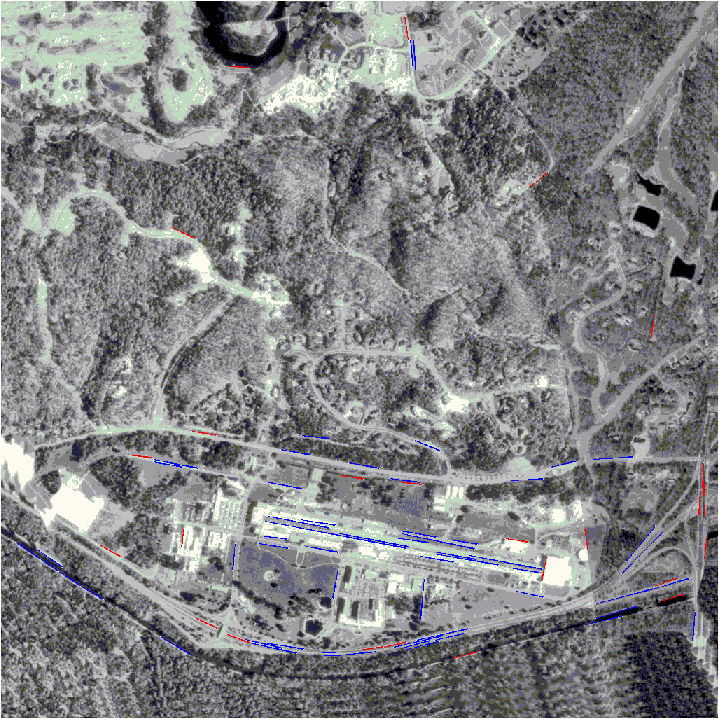
Figure 7 Lines detected
in second image
The lines detected in the second source image are shown above, overlaid on the
original. The lines that are below threshold are colored red, and the lines
used are in blue.

Figure
8 Lines from both images
The lines from both images are shown together in the above image (green for
the first image, blue for the second). Only line lengths above the threshold
are shown.
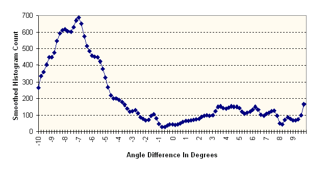
Figure 9 Angle Difference Histogram
The above figure shows the smoothed histogram of angle difference values. Based
on the peak value in the bin at -7, this value was chosen to be the rotational
angle between images.

Figure 10 Lines from
both images after derotation
The lines from both images are shown again, after the lines in the second image
(blue) are rotated to remove the rotational difference between the two images.
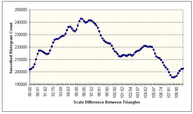
Figure 11 Scale Difference Histogram
The above figure shows the smoothed histogram of relative scales of the triangles.
Based on the peak value in the bin at 96.16%, this value was chosen to be the
scale factor between images.
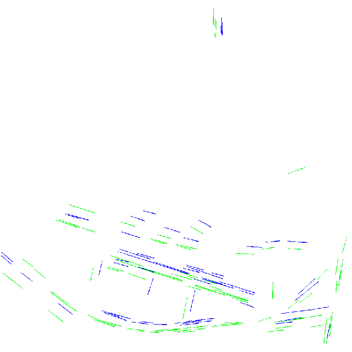
Figure 12 Lines from both images after descaling
The line pairs are shown above after compensation for the second image's scaling
factor.
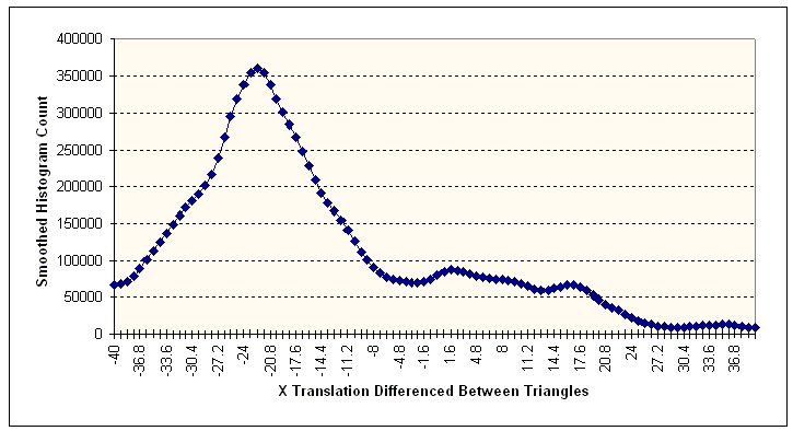
Figure 13 Translation Values in X
The above figure shows the smoothed histogram of the translation values in the
X axis between the set of triangles. Based on the peak at -22.4, this value
was chosen to be the translation on the X axis.
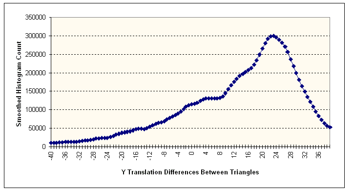
Figure 14 Translation Values In
Y
The above figure shows the smoothed histogram of the translation values in the
Y axis between the set of triangles. Based on the peak at 23.2, this value was
chosen to be the translation on the Y axis.
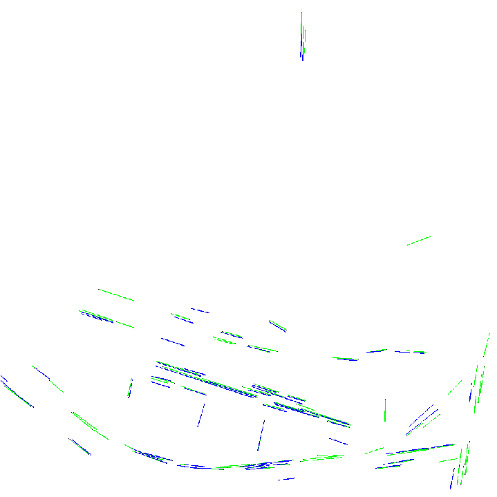
Figure 15 Lines from
both images after detranslation
The above image shows the lines after removing the translation factors determined
by the program.
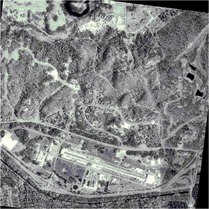
Figure 16 Second
image transformed to correspond to first
The above image shows the final result of the process: the second image transformed
such that it corresponds to the first image.

Figure 17 Difference
image of result and ortho1.pgm
The difference image between the original and output images is shown above (where
white is no difference, black is maximal difference). The areas of maximum difference
are the regions in the output image that mapped to areas outside the original
second image, and so were colored black.
Page created by
Les
Elkins on 4/15/96